Numerics & Simulations
Mathematical Framework & Numerical Methods
1. The Dispersive-Hyperbolic Model
Click to view Governing Equations & Variable Definitions
The physical setup and variable definitions are illustrated below: 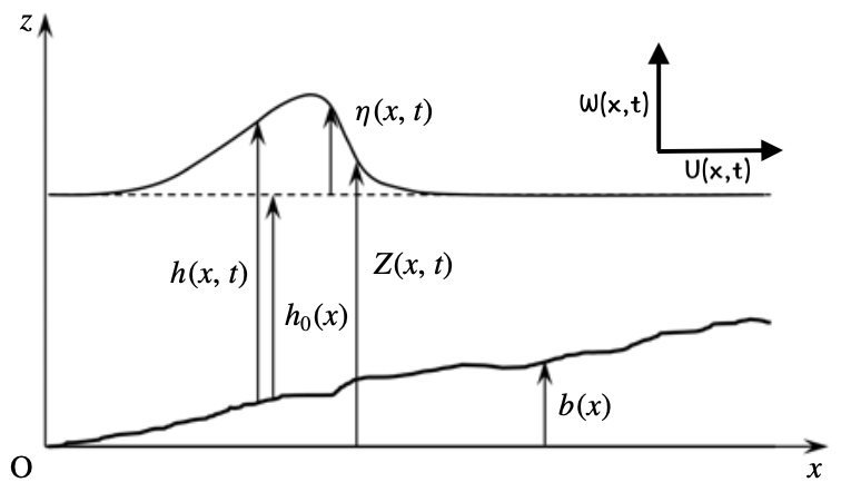
Figure 1: Definition of physical variables and coordinate system for the depth-averaged model.
The governing system is formulated as follows:
Where:
- \(h\): The water depth.
- \(U, W\): Depth-averaged horizontal and vertical velocity, respectively.
- \(P\): Depth-averaged non-hydrostatic pressure.
- \(\varphi\): Enstrophy, tracking the vorticity magnitude in the fluid.
- \(a_c\): Acoustic sound velocity (for the pressure wave) (chosen value).
- \(\langle P^r\rangle\): Energy dissipation due to wave breaking.
- \(\nu_T\): Turbulent viscosity.
Note: \(\langle P^r\rangle = \langle P^r\rangle(\varphi)\) and \(\nu_T = \nu_T(\varphi)\) are functions of enstrophy \(\varphi\).
2. Improved Dispersive Properties
Click to view the model with improved dispersive properties
The dispersive properties is improved adapting the method of Bonneton et al., 2011, where instead of the depth-averaged vertical velocity, one uses
The improved governing system is then written as:
Where:
- \(S\): Analogue to the gradient of \(Z\).
- \(\alpha\): A constant affecting the dispersive properties (an optimal value of \(1.159\) was found by Bonneton et al., 2011).
3. Numerical Implementation
Click to view Numerical methods & Treatment of breaking
To solve numerically the system of partial differential equations (PDEs), I implement second-order schemes designed for conservation laws:
- Spatial Discretization: Monotone Upstream Centered Scheme for Conservation Laws (MUSCL) with Rusanov flux and without slope limiter.
- Temporal Integration: Diagonally-implicit Runge-Kutta (DIRK) Implicit-Explicit (IMEX) ARS2(2,2,2) for second-order time accuracy.
- Well-Balanced Property: Ensuring the scheme preserves the “lake-at-rest” steady state over complex, non-flat bathymetry.
- Treatment of breaking: A novel breaking criterion related to the enstrophy was proposed by Kazakova & Richard, 2019, where a variable analogous to the enstrophy, called the virtual enstrophy \(\psi\), is solved by an identical enstrophy equation in parallel with the original equations, to avoid introducing sudden strong discontinuity to the system when breaking happens.
When there is , the model solves:
\(\varphi\) remains zero or constant while \(\psi\) tracks the potential breaking intensity.
$$ \begin{aligned} &\frac{\partial h}{\partial t}+\frac{\partial hU}{\partial x} = 0\\ &\frac{\partial hU}{\partial t}+\frac{\partial}{\partial x}\left(hU^2+\frac{gh^2}{2}+h^3\varphi+hP\right)= -gh\frac{\partial b}{\partial x}\\ &\frac{\partial hW^\ast}{\partial t}+\frac{\partial hUW^\ast}{\partial x} = \frac{3}{2}P+4\frac{\alpha-1}{\alpha^2}{W^{\ast}}^2+\frac{\alpha-1}{2\alpha}gh^2\frac{\partial S}{\partial x}\\ &\frac{\partial hP}{\partial t}+\frac{\partial hUP}{\partial x} = -a_c^2\left(\alpha h\frac{\partial U}{\partial x}+2W^\ast\right)\\ &\frac{\partial hS}{\partial t}+\frac{\partial hUS}{\partial x} = 2h\frac{\partial W^\ast}{\partial x}+\frac{2}{\alpha}W^\ast S\\ &\frac{\partial h\varphi}{\partial t}+\frac{\partial hU\varphi}{\partial x} = -\frac{2}{h}\langle P^r\rangle(\varphi) \\ &\frac{\partial h\psi}{\partial t}+\frac{\partial hU\psi}{\partial x} = -\frac{2}{h}\langle P^r\rangle(\psi)+\frac{4\nu_T(\psi)}{h}\left(\frac{\partial U}{\partial x}\right)^2-\frac{8\nu_T(\psi)W^\ast}{\alpha^2h^2}\frac{\partial U}{\partial x} \end{aligned} $$4. Breaking criterion
Click to view Breaking criterion
To accurately determine the breaking zone, a revised breaking criterion is implemented to the 1D model based on the transition between two state-dependent quantities:
The triggering mechanism is governed by two thresholds, \(\psi_0 > \psi_1 \geq 0\), which define the activation and deactivation phases:
- Activation: Breaking is initiated when \(\widetilde{\psi_\eta} > \psi_0\).
- Persistence: Once active, the breaking state is maintained as long as \(\widetilde{\psi_h} > \psi_1\).
Furthermore, the location of turbulence generation and vortex generation for a plunging breaker is mainly in the front part of the wave. To ensure the numerical model reflects this spatial localization, a constraint is applied to the breaking zone:
The thresholds were determined by fitting an empirical law to experimental data as a function of the bed slope \(\tan\beta\).
Simulations
The following simulations are based on the improved dispersive model. In the following simulation, the zone where the activation criterion is met is indicated by the translucent red zone. The true breaking region (not shown here), where dissipative terms are activated, is much narrower and localized at the wave front.
1. Solitary wave propagation over flat bed
In the experiment of Watanabe et al., 2001, the physical limit of solitary wave stability was investigated to determine the critical non-linearity at which a wave begins to break. The waves are characterized by the non-linearity parameter \(\mu = a/h\), amplitude over water depth.
Case A: Stable Solitary Wave (\(\mu = 0.66\))
Animation 1: Propagation of a stable solitary wave (\(\mu = 0.66\)).
Case B: Unstable Solitary Wave (\(\mu = 0.78064\))
Animation 2: Spontaneous breaking of an unstable solitary wave (\(\mu = 0.78064\)).
2. Solitary wave propagation over a slope
In the experiment of Hsiao et al., 2008, a solitary wave of amplitude \(a_\ast\) is generated and propagates over the topography of slope \(\beta\) with \(\tan \beta = 1/60\) at a given still water level \(h_0\). The experiment consists of 54 trials with different choices of still water level \(h_0\) and nonlinearity parameter \(\mu = a_\ast/h_0\) from which the wave amplitude can be calculated. The following simulation and gauge point comparison are from trial 41, where \(h_0 = 2.2\) m and \(\mu = 0.137\) were chosen.
Animation 3: Solitary wave \(\mu = 0.137\) propagation over a slope \(\tan \beta = 1/60\).
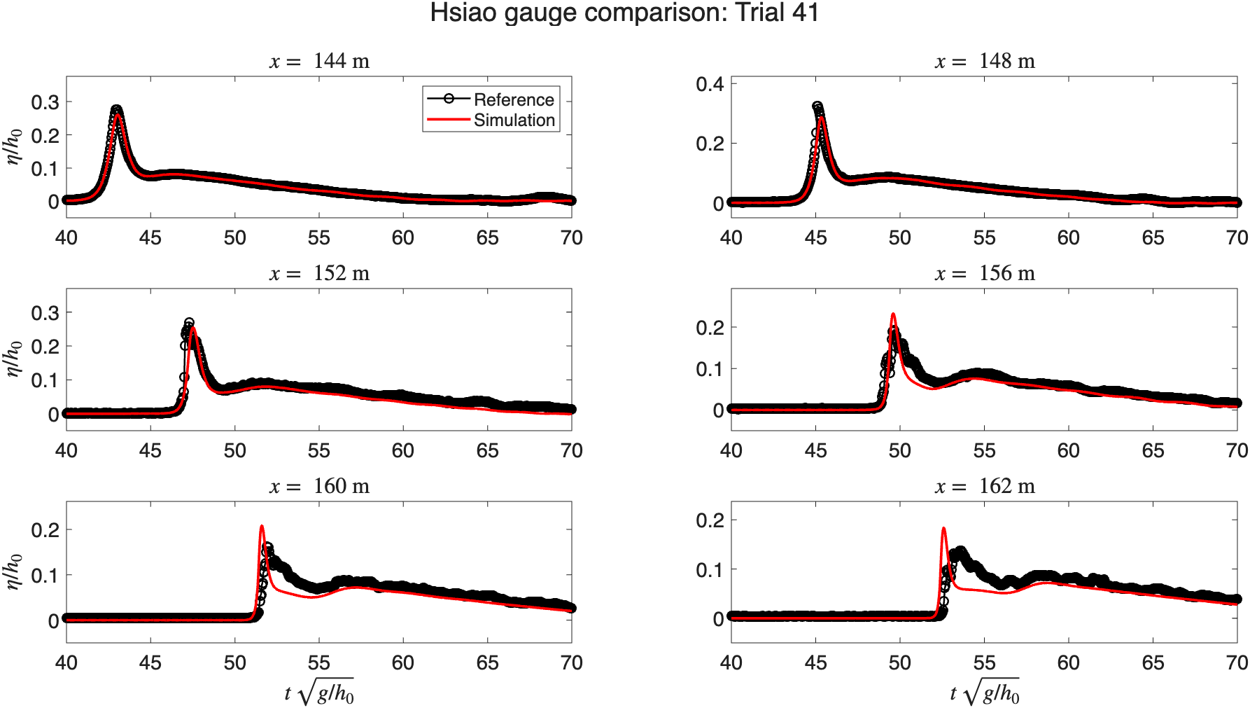
Figure 2: Time series of free surface elevation at multiple gauge locations for Trial 41. Solid red lines represent numerical results, and black circles/lines denote experimental data.
3. Wavetrain propagation
This section presents two simulations of wave train propagation. The first case replicates the experiment by Cox, 1995, in which a wave train with \(a_\ast = 0.115\) m and \(T = 2.2\) s propagates over a \(1/35\) slope. The six gauge locations are marked by solid vertical lines in the simulation below.
Animation 4: Wave train propagation over a slope \(\tan \beta = 1/35\). The solid vertical lines indicate the locations of the six gauges. A 7.5-meter-wide absorbing layer is applied to the right boundary of the domain.
The time series of free surface elevation at the six gauge points are shown in the figure below.
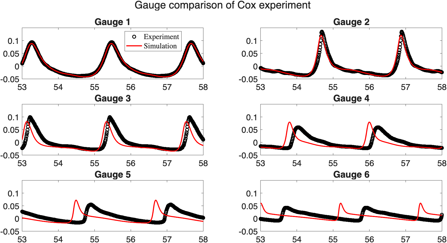
Figure 3: Time series of free surface elevation at six gauge points. Solid red lines represent numerical results, and black circles denote experimental data.
The second case focuses on the experiment of Beji & Battjes, 1993, in which regular sinusoidal wave trains are generated and propagate over a submerged bar. The regular sinusoidal wave train with period \(T = 2.5\) s and amplitudes \(a_\ast = 0.022\) m are generated (spilling breaker type). A 5 m sponge layer is applied on the right side of the domain to absorb outgoing waves and the incoming wave is generated on the left side as a Dirichlet boundary condition. The eight gauge locations are marked by solid vertical lines in the simulation below.
Animation 5: Wave train propagation over a submerged bar. The solid vertical lines indicate the locations of the eight gauges.
The time series of free surface elevation at the eight gauge points are shown in the figure below.
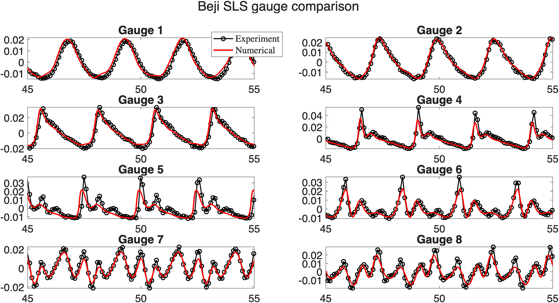
Figure 4: Time series of free surface elevation at eight gauge points of the regular wave train. Solid red lines represent numerical results, and black circles denote experimental data.